PureData Objects with Python

With the py4pd it is possible to create new PureData objects using Python. For that, you need to declare your Python functions and then create a function called py4pdLoadObjects. See the Python Code:

Breaking Changes

I had change how pd.addobject work from version 0.6 to version 0.7. Now, me use the function and the Pure Data object. Instead of use this, pd.addobject("mysumObject", "NORMAL", "myNewPdObjects", "mysumObject") we use this pd.addobject(mysumObject, "mysumObject")

myNewPdObjects.py

import pd

def mysumObject(a, b, c, d):
    return a + b + c + d

def py4pdLoadObjects():
    pd.addobject(mysumObject, "mysumObject") # function, string with name of the object

    # My License, Name and University, others information
    pd.print("", show_prefix=False)
    pd.print("GPL3 | by Charles K. Neimog", show_prefix=False)
    pd.print("University of São Paulo", show_prefix=False)
    pd.print("", show_prefix=False)

In the code above, we create a new object called mysymObject. It is saved inside an script called myNewPdObjects.py. To load this script in PureData how need to follow these steps:

• Copy the script myNewPdObjects.py for the resources/scripts inside py4pd folder or put it on side of your PureData patch.
• Create a new py4pd with this config: py4pd -library myNewPdObjects.
• Add the new object, in this case mysumObject.

Following this steps we have this patch:

Note that we need to declare py4pd -library or py4pd -lib as is used in declare object, followed by the name of the script where the function py4pdLoadObjects is located.

If you have some problem to do that, please report on Github.

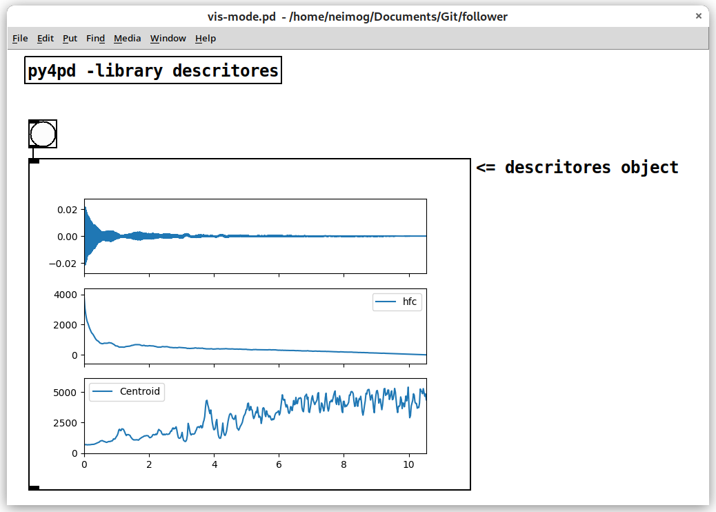
Visualization Mode for Objects

You can create new Visualization modes for Objects, for that you have the option of two keyword: objtype and figsize. See the example where I define one function use to see graphs.

import pd
import audioflux as af
import matplotlib.pyplot as plt
from audioflux.display import fill_plot, fill_wave
from audioflux.type import SpectralFilterBankScaleType, SpectralDataType
import numpy as np

def descriptors():
    audio_arr, sr = af.read(pd.home() + "/Hp-ord-A4-mf-N-N.wav")
    bft_obj = af.BFT(num=2049, samplate=sr, radix2_exp=12, slide_length=1024,
                   data_type=SpectralDataType.MAG,
                   scale_type=SpectralFilterBankScaleType.LINEAR)
    spec_arr = bft_obj.bft(audio_arr)
    spec_arr = np.abs(spec_arr)
    spectral_obj = af.Spectral(num=bft_obj.num,
                               fre_band_arr=bft_obj.get_fre_band_arr())
    n_time = spec_arr.shape[-1]  # Or use bft_obj.cal_time_length(audio_arr.shape[-1])
    spectral_obj.set_time_length(n_time)
    hfc_arr = spectral_obj.hfc(spec_arr)
    cen_arr = spectral_obj.centroid(spec_arr) 

    fig, ax = plt.subplots(nrows=3, sharex=True)
    fill_wave(audio_arr, samplate=sr, axes=ax[0])
    times = np.arange(0, len(hfc_arr)) * (bft_obj.slide_length / bft_obj.samplate)
    fill_plot(times, hfc_arr, axes=ax[1], label='hfc')
    fill_plot(times, cen_arr, axes=ax[2], label="Centroid")
    tempfile = pd.tempfolder() + "/descritores.png"
    plt.savefig(tempfile)
    pd.show(tempfile)
    pd.print("Data plotted")

def py4pdLoadObjects():
    pd.addobject(descriptors, "descritores", objtype="VIS", figsize=(640, 480))

See the result: